What is Recurrent Neural Network (RNN)?

Neural networks are widely used in artificial intelligence to identify patterns and relationships in data. However, traditional neural networks like feedforward networks struggle with sequential data—information where the order of inputs matters, such as sentences, time-series data, or speech.

Recurrent Neural Networks (RNNs) address this limitation by retaining information from previous steps through an internal state, enabling them to process sequences of data step-by-step. This makes RNNs ideal for tasks like language modeling, speech recognition, and machine translation, where context from earlier inputs is essential for accurate predictions. Unlike standard neural networks, RNNs can store memory over time through feedback loops, making them effective for sequential tasks.

What is a recurrent neural network (RNN)?

At its core, a Recurrent Neural Network (RNN) is a type of neural network specifically designed to handle sequential data by maintaining memory of previous inputs through an internal hidden state. Think of it like a conveyor belt that retains information from each step, using it to influence future steps.

Key Concept

• Hidden State: At each step, the RNN processes the current input along with the hidden state (which contains information from previous steps). This feedback loop allows it to remember past data points and apply that knowledge to make better predictions at the next time step.

For example, in language models, when predicting the next word in a sentence like “I am feeling under the …”, the RNN uses the words it has already seen (“I am feeling under”) to predict that the next word is likely “weather”​

Why RNNs are Different

• RNNs share parameters across different time steps, which makes them more efficient when dealing with sequential data compared to traditional feedforward networks, where each layer has its own parameters.
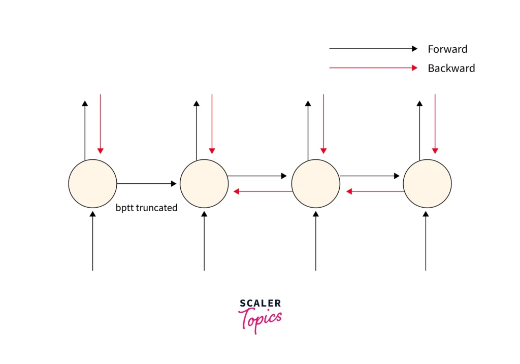
• They leverage Backpropagation Through Time (BPTT), a training algorithm that adjusts weights by summing up errors over each time step, ensuring that both past and current states contribute to the model’s learning.

How RNNs Work

An RNN’s architecture can be visualized as a series of connected units, each passing information to the next. At each time step, an RNN takes both the current input and the hidden state from the previous step as inputs, processes them, and produces a new hidden state and output. This recurrent nature allows the network to retain information over time and make predictions based on both past and current data.

The Architecture of an RNN

• Unfolded RNN Diagram: When unfolded over time, an RNN looks like a sequence of neural network layers where each layer corresponds to a time step. The key is that the hidden state (memory) carries information across these time steps.

Mathematical Operations:

At each time step $t$, the following operations occur:

1. Updating the Hidden State:

$h_t = \sigma(W_h \cdot h_{t-1} + W_x \cdot x_t + b)$

• $h_t$: Current hidden state
• $h_{t-1}$: Hidden state from the previous step
• $x_t$: Input at time $t$
• $W_h$ and $W_x$: Weight matrices
• $b$: Bias
• $\sigma$: Activation function (e.g., Tanh or ReLU)

2. Generating the Output:

$y_t = W_y \cdot h_t + c$

• $y_t$: Output at time $t$
• $W_y$: Output weight matrix
• $c$: Output bias

Training with Backpropagation Through Time (BPTT):

Training an RNN involves BPTT (Backpropagation Through Time). This algorithm adjusts the weights by computing gradients over multiple time steps. However, due to the sequential nature of RNNs, they often suffer from vanishing or exploding gradients, making it difficult to learn long-term dependencies​.

Types of RNNs

RNNs come in several variants, each designed to handle different types of input and output sequences. Below are the common types of RNNs based on input-output configurations:

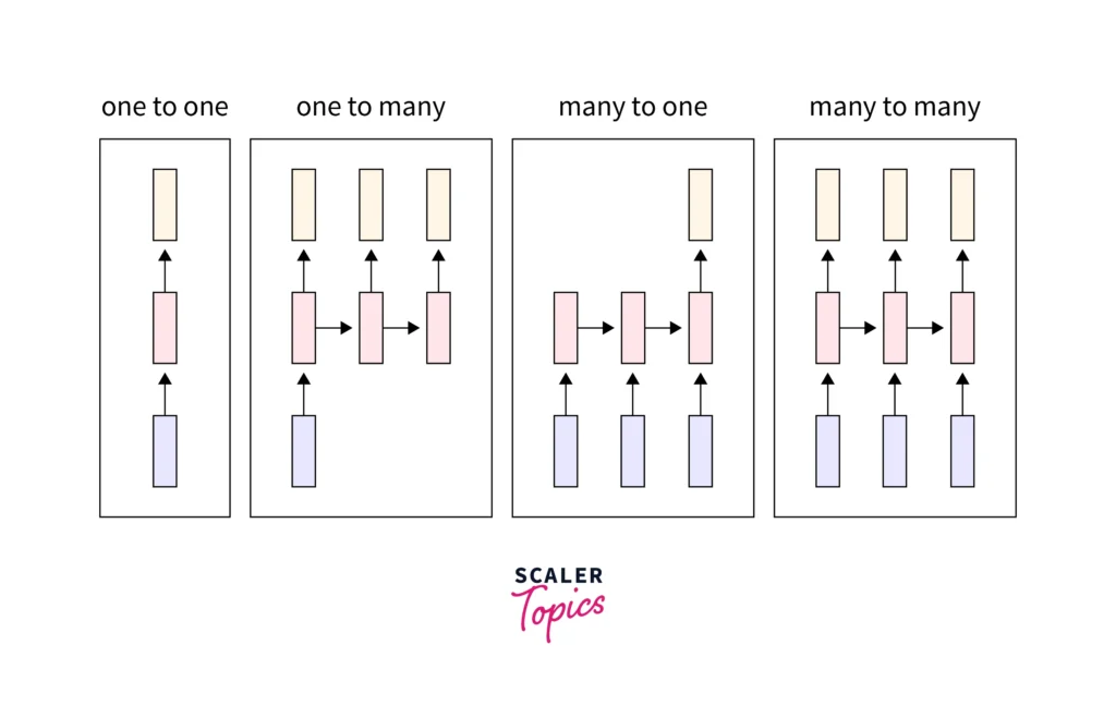
1. One-to-One:
   • This is the simplest form of RNN, where one input corresponds to one output.
   • Example: Binary classification tasks, such as determining if an email is spam or not.
2. One-to-Many:
   • A single input generates multiple outputs.
   • Example: Generating a sequence of words from an image (image captioning).
3. Many-to-One:
   • Multiple inputs lead to a single output.
   • Example: Sentiment analysis, where a sequence of words is used to predict a single sentiment (positive/negative).
4. Many-to-Many:
   • Both the inputs and outputs are sequences.
   • Example: Machine translation, where a sentence in one language is converted into another language.

These configurations allow RNNs to be applied flexibly across a variety of use cases, such as speech-to-text, chatbots, and time-series forecasting

How does RNN Differ from Feedforward Neural Network?

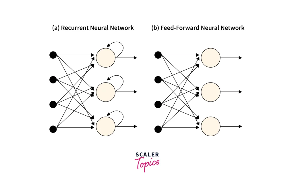
The key difference between Recurrent Neural Networks (RNNs) and Feedforward Neural Networks (FNNs) lies in how information flows through the network.

1. Information Flow:
   • In a Feedforward Neural Network (FNN), the data flows in a single direction, from the input layer to the output layer, without loops or feedback.
   • In an RNN, information flows both forward and through recurrent loops, enabling it to retain memory of previous inputs.
2. Handling of Sequential Data:
   • FNNs process inputs independently, meaning they cannot retain context across time steps.
   • RNNs store information in hidden states and use past inputs to influence future outputs, making them better suited for sequential data tasks, such as time-series forecasting, language modeling, or speech recognition.
3. Use Cases:
   • FNNs work well for tasks like image classification, where the data points are independent.
   • RNNs excel in problems where the order of inputs matters, such as sentence generation or stock price prediction.

Common Activation Functions

Activation functions are essential in RNNs because they introduce non-linearity, enabling the network to learn complex patterns in sequential data. Below are the most common activation functions used in RNNs:

1. Sigmoid Function

$\sigma(x) = \frac{1}{1 + e^{-x}}$

• Range: $0$ to $1$
• Use Case: Controls gates in LSTMs to decide how much information to retain or forget.
• Limitation: Prone to the vanishing gradient problem, making it less ideal for deeper networks.

2. Tanh (Hyperbolic Tangent) Function

$\tanh(x) = \frac{e^x – e^{-x}}{e^x + e^{-x}}$

• Range: $-1$ to $1$
• Use Case: Often preferred over Sigmoid because it outputs values centered around 0, leading to smoother gradient flow.
• Limitation: Still susceptible to the vanishing gradient problem, though less severe than Sigmoid.

3. ReLU (Rectified Linear Unit)

$f(x) = \max(0, x)$

• Range: $0$ to$ ∞$
• Use Case: Speeds up training by avoiding saturation, making it a popular choice in deep learning.
• Limitation: Can suffer from the exploding gradient problem, especially in RNNs due to unbounded outputs. Variants like Leaky ReLU and Parametric ReLU are used to mitigate this.

Architecture Variants of Recurrent Neural Network

Several variants of RNNs have been developed to address specific challenges, such as vanishing gradients or the need for better sequence learning. Below are the most common types:

1. Standard RNNs

• The basic version of an RNN processes input sequentially, using the current input and the previous hidden state to generate the next hidden state.
• Limitation: It struggles with learning long-term dependencies due to the vanishing gradient problem.

2. Bidirectional RNNs (BRNNs)

• BRNNs process data in both forward and backward directions, enabling them to use both past and future context.
• Use Case: Helpful in tasks like speech recognition where both previous and upcoming words are relevant for accurate predictions.

3. Long Short-Term Memory Networks (LSTMs)

• LSTMs address the vanishing gradient problem by introducing memory cells with three gates:
  • Input Gate: Controls how much new information enters the cell.
  • Forget Gate: Decides what information to discard.
  • Output Gate: Controls what information to pass to the next step.
• Use Case: Widely used in tasks that require learning long-term dependencies, such as language modeling and machine translation.

4. Gated Recurrent Units (GRUs)

• GRUs are a simpler alternative to LSTMs, with only two gates:
  • Reset Gate: Controls how much past information to forget.
  • Update Gate: Determines how much of the new input to retain.
• Use Case: GRUs are faster to train and perform well in resource-constrained environments.

5. Encoder-Decoder RNNs

• Encoder-decoder RNNs are designed for sequence-to-sequence tasks, such as machine translation.
• The encoder processes the input sequence into a fixed-length vector, while the decoder uses that vector to generate the output sequence.
• Limitation: Managing long input sequences with a fixed-length vector can become a bottleneck.

Advantages and Limitations of RNNs

Advantages of RNNs

1. Sequential Data Handling:
   • RNNs excel at tasks where the order of inputs matters, such as time-series forecasting, speech recognition, and text generation.
2. Memory Retention:
   • Through their hidden state, RNNs can retain information from previous steps, making them suitable for tasks requiring contextual understanding.
3. Parameter Sharing Across Time Steps:
   • RNNs use the same parameters across all time steps, reducing the complexity of the model and making it computationally efficient​.
4. Real-time Data Processing:
   • RNNs can process input sequences in real-time, which is beneficial in applications like chatbots and sensor data analysis.

Limitations of RNNs

1. Vanishing and Exploding Gradients:
   • When processing long sequences, gradients can either become too small (vanishing) or too large (exploding), making it difficult for the model to learn effectively.
2. Limited Long-term Memory:
   • Standard RNNs struggle to remember dependencies that span across many time steps, leading to poor performance in tasks requiring long-term context.
3. Training Complexity:
   • Training RNNs can be slow due to the sequential nature of processing and backpropagation through time (BPTT).
4. Replaced by Advanced Architectures:
   • With the rise of transformers (like BERT and GPT), which handle sequential data more efficiently, RNNs are becoming less common in modern applications.

RNN Code Implementation

When implementing RNNs, several deep learning frameworks offer easy-to-use tools. Here are the commonly used libraries:

Imported Libraries

• TensorFlow: A popular deep learning framework that simplifies RNN creation through Keras.
• PyTorch: A flexible framework known for real-time and research-based applications.
• Keras: A high-level neural network API, now integrated into TensorFlow, perfect for rapid prototyping.

1. Input Generation

Prepare the dataset. For example, convert time-series data into sequences.

X_train, y_train = generate_sequences(data, sequence_length=10)

2. Model Building

Create the RNN architecture using TensorFlow/Keras.

from tensorflow.keras.models import Sequential
from tensorflow.keras.layers import SimpleRNN, Dense

# Initialize the model
model = Sequential()

# Add an RNN layer with 50 units and 'tanh' activation
model.add(SimpleRNN(50, activation='tanh', input_shape=(10, 1)))

# Add an output layer with a single neuron
model.add(Dense(1))

3. Model Compilation

Compile the model with an optimizer and loss function.

model.compile(optimizer='adam', loss='mse', metrics=['accuracy'])

4. Model Training

Train the model with training data.

model.fit(X_train, y_train, epochs=10, batch_size=32)

5. Model Prediction and Output

Use the trained model to make predictions.

y_pred = model.predict(X_test)
print("Predicted Output:\n", y_pred)

Sample Output:

Predicted Output:
 [[0.412]
 [0.376]
 [0.598]
 [0.245]]

In this example, the RNN generates predictions for the input sequences, where each output corresponds to a time step prediction. The values are typically normalized or scaled based on the problem domain.

Conclusion

Recurrent Neural Networks (RNNs) are powerful models designed to handle sequential data, making them ideal for applications like text generation, speech recognition, and time-series forecasting. With their ability to retain memory through hidden states, RNNs excel in learning from context and predicting future steps based on past inputs. However, challenges like vanishing gradients and long-term dependency issues highlight the importance of advanced architectures like LSTMs and GRUs.

Despite recent advances with transformer models, RNNs remain a crucial tool for sequential data tasks due to their simplicity and real-time processing capabilities. By leveraging frameworks such as TensorFlow, PyTorch, and Keras, RNNs can be easily implemented, trained, and deployed for practical use cases.