Naive Bayes Algorithm Classifier in Machine Learning

In machine learning, classification problems are essential for making decisions, like predicting whether an email is spam or not. One of the simplest and most popular algorithms for classification is the Naive Bayes classifier. This algorithm is widely used because of its simplicity, speed, and efficiency, even when dealing with large datasets.

The Naive Bayes algorithm plays a key role in applications such as spam detection, sentiment analysis, and recommendation systems. Understanding how it works and when to use it can greatly help beginners entering the world of machine learning.

What is Naive Bayes Classifier?

The Naive Bayes classifier is a supervised learning algorithm used for solving classification problems. It is based on Bayes’ Theorem, which calculates the probability of a certain event occurring based on prior knowledge. The Naive Bayes algorithm assigns new data points to the most likely class by comparing probabilities.

The algorithm is widely used in real-world scenarios, such as classifying emails into spam and non-spam or identifying the sentiment of customer reviews. The strength of this algorithm lies in how efficiently it handles data, even with limited training examples.

Why is it called Naive Bayes?

The Naive Bayes algorithm is called “naive” because it makes a strong assumption: all the features in the dataset are independent of each other. This means that the presence of one feature does not affect the presence of another.

In reality, many features are correlated, and this assumption may not always hold. However, despite this simplification, the Naive Bayes algorithm often performs well in practice. Its simplicity allows for quick computation, making it a popular choice for tasks like text classification and spam detection.

Dataset

Consider a fictional dataset that describes the weather conditions for playing a game of golf. Each row in the dataset records the weather, temperature, and whether the conditions were suitable for playing. The goal is to predict whether it’s fit (“Yes”) or unfit (“No”) for playing golf based on the weather conditions. Below is a tabular representation of our dataset.

Weather	Temperature	Play?
Sunny	Hot	No
Sunny	Hot	No
Overcast	Hot	Yes
Rainy	Mild	Yes
Rainy	Cool	Yes
Rainy	Cool	No
Overcast	Cool	Yes
Sunny	Mild	No
Sunny	Cool	Yes
Rainy	Mild	Yes
Sunny	Mild	Yes
Overcast	Mild	Yes
Overcast	Hot	Yes
Rainy	Mild	No

This dataset provides a simple example to illustrate how the Naive Bayes classifier calculates probabilities. Later in the article, we will use this dataset to walk through examples and the algorithm implementation.

Bayes’ Theorem

Bayes’ Theorem is a fundamental concept that forms the basis of the Naive Bayes algorithm. It calculates the posterior probability of an event occurring based on prior knowledge and evidence. In simple terms, it helps answer: “Given some observations, how likely is this event to belong to a particular class?”

The mathematical formula for Bayes’ Theorem is:

$ P(A \mid B) = \frac{P(B \mid A) \times P(A)}{P(B)} $

Where:

• P(A∣B): Posterior probability – probability of hypothesis A given that B is true.
• P(B∣A): Likelihood – probability of observing B given that A is true.
• P(A): Prior probability – the initial probability of A before seeing any evidence.
• P(B): Marginal probability of observing B.

How Bayes’ Theorem Works in Naive Bayes Classifier

In a Naive Bayes classifier, Bayes’ Theorem is used to calculate the probability of a class based on given features. For instance, if we want to predict whether it is fit to play golf on a Sunny day with Mild temperature, the classifier will compute two probabilities:

1. P(Play = Yes | Sunny, Mild) – Probability of playing on a sunny, mild day.
2. P(Play = No | Sunny, Mild) – Probability of not playing on a sunny, mild day.

Whichever probability is higher becomes the final prediction.

Naive Assumption

In the Naive Bayes algorithm, we assume that all features are independent of each other, which simplifies the computation. This is known as the “naive” assumption. Although this assumption may not always be true in practice, it often leads to good results.

Simplified Example Calculation

Let’s consider our dataset. To compute the probability of Play = Yes on a Sunny day with Mild temperature, we need the following:

$ P(\text{Play}=\text{Yes} \mid \text{Sunny}, \text{Mild}) = \frac{P(\text{Sunny} \mid \text{Play}=\text{Yes}) \times P(\text{Mild} \mid \text{Play}=\text{Yes}) \times P(\text{Play}=\text{Yes})}{P(\text{Sunny}, \text{Mild})} $

Similarly, the algorithm will calculate P(Play = No | Sunny, Mild). The class with the higher probability will be the predicted outcome.

Bayes’ Theorem: Implementation (Example)

To demonstrate how Bayes’ Theorem works, let’s predict whether we can play outside on a sunny day with mild temperature using the dataset.

The dataset has two features: Weather (Sunny, Overcast, Rainy) and Temperature (Hot, Mild, Cool). The target variable is Play (Yes/No). We’ll calculate the probabilities step by step.

Goal:

Predict if Play = Yes or Play = No for Weather = Sunny and Temperature = Mild.

Step 1: Calculate Prior Probabilities

We first calculate the prior probabilities for each class:

$ P(\text{Play}=\text{Yes}) = \frac{\text{Number of Yes outcomes}}{\text{Total number of outcomes}} = \frac{9}{14} $

$ P(\text{Play}=\text{No}) = \frac{5}{14} $

Step 2: Calculate Likelihood Probabilities

Next, we calculate the likelihood probabilities for each feature value based on the given class:

• For Weather = Sunny:

$ P(\text{Sunny} \mid \text{Play}=\text{Yes}) = \frac{\text{Sunny and Play = Yes}}{\text{Total Yes outcomes}} = \frac{2}{9} $

$ P(\text{Sunny} \mid \text{Play}=\text{No}) = \frac{3}{5} $

• For Temperature = Mild:

$ P(\text{Mild} \mid \text{Play}=\text{Yes}) = \frac{\text{Mild and Play = Yes}}{\text{Total Yes outcomes}} = \frac{4}{9} $

$ P(\text{Mild} \mid \text{Play}=\text{No}) = \frac{2}{5} $

Step 3: Apply Bayes’ Theorem

Now, we calculate the posterior probabilities for both classes using Bayes’ Theorem.

$ P(\text{Play} = \text{Yes} \mid \text{Sunny}, \text{Mild}) = \frac{2}{9} \times \frac{4}{9} \times \frac{9}{14} $

$ P(\text{Play} = \text{Yes} \mid \text{Sunny}, \text{Mild}) = \frac{8}{126} = 0.0635 $

Similarly, we calculate the probability for Play = No:

$$ P(\text{Play}=\text{No} \mid \text{Sunny}, \text{Mild}) = P(\text{Sunny} \mid \text{Play}=\text{No}) \times P(\text{Mild} \mid \text{Play}=\text{No}) \times P(\text{Play}=\text{No}) $$

$ P(\text{Play}=\text{No} \mid \text{Sunny}, \text{Mild}) = \frac{3}{5} \times \frac{2}{5} \times \frac{5}{14} = \frac{30}{350} = 0.0857 $

Step 4: Make the Prediction

Since P(Play = No | Sunny, Mild) is greater than P(Play = Yes | Sunny, Mild), the classifier will predict:

Prediction: Play = No

Working of Naive Bayes Classifier

The Naive Bayes classifier works in two main stages: training and prediction. Below is a step-by-step breakdown of how the algorithm classifies new data using the dataset we introduced earlier.

Step 1: Training the Model

In the training phase, the algorithm calculates:

1. Prior Probability:

The probability of each class in the dataset.

Example:

$ P(\text{Play}=\text{Yes}) = \frac{\text{Number of Yes outcomes}}{\text{Total number of outcomes}} = \frac{9}{14} $

$ P(\text{Play}=\text{No}) = \frac{5}{14} $

2. Conditional Probability:

The probability of each feature value given a class.

Example:

$ P(\text{Sunny} \mid \text{Play}=\text{Yes}) = \frac{\text{Number of Sunny days when Play=Yes}}{\text{Total Yes outcomes}} = \frac{2}{9} $

$ P(\text{Sunny} \mid \text{Play}=\text{No}) = \frac{3}{5} $

3. Smoothing (Optional):

If a feature value has zero occurrences for a class, it can make the probability zero. Smoothing techniques like Laplace Smoothing are used to handle this.

Step 2: Making Predictions

To predict the class of a new data point (e.g., a Sunny day with Mild temperature), the classifier calculates the posterior probability for each class.

$ P(\text{Play}=\text{Yes} \mid \text{Sunny}, \text{Mild}) = P(\text{Sunny} \mid \text{Play}=\text{Yes}) \times P(\text{Mild} \mid \text{Play}=\text{Yes}) \times P(\text{Play}=\text{Yes}) $

Similarly:

$ P(\text{Play}=\text{No} \mid \text{Sunny}, \text{Mild}) = P(\text{Sunny} \mid \text{Play}=\text{No}) \times P(\text{Mild} \mid \text{Play}=\text{No}) \times P(\text{Play}=\text{No}) $

The classifier will select the class with the highest probability as the prediction.

Summary of the Workflow

1. Training Phase: Calculate prior and conditional probabilities from the dataset.
2. Prediction Phase: Use Bayes’ Theorem to find the class with the highest probability.
3. Output: The predicted class is assigned to the new data point.

Advantages of Naive Bayes Classifier

• Simplicity and Ease of Implementation: Naive Bayes is straightforward to implement and requires less computational power compared to other algorithms.
• Fast Training and Prediction: Since it involves simple probability calculations, Naive Bayes is efficient for both training and making predictions, even on large datasets.
• Performs Well with High-Dimensional Data: The algorithm works effectively even with datasets that contain many features, such as text classification where each word becomes a feature.
• Works Well with Small Datasets: Naive Bayes can perform reliably even with limited training data, as it generalizes well using prior probabilities.
• Handles Categorical and Text Data: It is widely used in spam filtering, sentiment analysis, and news classification due to its efficiency with categorical data.

Disadvantages of Naive Bayes Classifier

• Naive Assumption of Feature Independence: The algorithm assumes that all features are independent of each other, which is rarely true in real-world datasets. This can reduce its accuracy if the features are highly correlated.
• Zero Probability Issue: If a feature value does not appear in the training data for a given class, the algorithm assigns zero probability to that class. This can be mitigated using Laplace Smoothing.
• Limited with Continuous Features: Naive Bayes struggles with continuous features unless they follow a normal distribution, as required in Gaussian Naive Bayes. Otherwise, data preprocessing may be necessary.
• Sensitive to Irrelevant Features: Including irrelevant or noisy features can negatively impact the classifier’s performance, as the algorithm gives equal importance to all features.
• Not Suitable for Complex Relationships: The algorithm may not perform well when there are complex relationships between features, as it lacks the capability to model feature interactions.

Applications of Naive Bayes Classifier

• Spam Filtering: Naive Bayes is at the heart of many spam detection systems. It classifies emails as spam or non-spam based on the occurrence of specific words or patterns.
• Sentiment Analysis: It is used to determine the sentiment of customer reviews, social media posts, or feedback by analyzing positive and negative words.
• Text Classification: Naive Bayes is effective for news categorization and classifying documents into categories like sports, technology, or politics.
• Recommendation Systems: It helps in building recommendation engines by predicting user preferences based on historical data.
• Medical Diagnosis: In healthcare, the algorithm can assist in predicting diseases based on patient symptoms and medical history.

Types of Naive Bayes Model

There are several variations of the Naive Bayes algorithm, each designed to handle specific types of data. Here are the most common types:

• Gaussian Naive Bayes (GNB):
  • Suitable for continuous features that follow a normal distribution (bell curve).
  • Example: Predicting stock prices or housing values using continuous data like price or area.
  • When to Use: Use when your features are continuous, like temperature or age, and follow a normal distribution.
• Multinomial Naive Bayes (MNB):
  • Works well with count data, where features represent the frequency of occurrences (e.g., word counts in text).
  • Example: Classifying documents or emails based on the frequency of words.
  • When to Use: Ideal for text classification tasks, such as spam detection, where features represent word frequencies.
• Bernoulli Naive Bayes (BNB):
  • Suitable for binary features (yes/no, true/false) where features can take only two values.
  • Example: Spam filtering, where words are either present (1) or absent (0) in an email.
  • When to Use: Best suited for tasks with binary features, such as sentiment analysis or spam filtering.

Python Implementation of the Naive Bayes Algorithm

In this section, we’ll walk through the step-by-step Python implementation of the Naive Bayes classifier using Scikit-learn, a popular machine learning library.

Step 1: Import Required Libraries

import pandas as pd
from sklearn.model_selection import train_test_split
from sklearn.naive_bayes import GaussianNB
from sklearn.metrics import accuracy_score, confusion_matrix

Step 2: Prepare the Dataset

For this example, let’s use a small dataset similar to the one introduced earlier. Here, we assume the data is available as a DataFrame.

# Create the dataset
data = {'Weather': ['Sunny', 'Sunny', 'Overcast', 'Rainy', 'Rainy', 'Rainy',
                    'Overcast', 'Sunny', 'Sunny', 'Rainy', 'Sunny', 'Overcast',
                    'Overcast', 'Rainy'],
        'Temperature': ['Hot', 'Hot', 'Hot', 'Mild', 'Cool', 'Cool', 'Cool',
                        'Mild', 'Cool', 'Mild', 'Mild', 'Mild', 'Hot', 'Mild'],
        'Play': ['No', 'No', 'Yes', 'Yes', 'Yes', 'No', 'Yes', 'No', 'Yes',
                 'Yes', 'Yes', 'Yes', 'Yes', 'No']}

# Convert to DataFrame
df = pd.DataFrame(data)

Step 3: Encode Categorical Features

Since Naive Bayes requires numerical input, we’ll convert the categorical data into numeric format.

from sklearn.preprocessing import LabelEncoder

le = LabelEncoder()
df['Weather'] = le.fit_transform(df['Weather'])
df['Temperature'] = le.fit_transform(df['Temperature'])
df['Play'] = le.fit_transform(df['Play'])

Step 4: Split the Data into Training and Testing Sets

X = df[['Weather', 'Temperature']]
y = df['Play']

X_train, X_test, y_train, y_test = train_test_split(X, y, test_size=0.3, random_state=42)

Step 5: Train the Naive Bayes Model

model = GaussianNB()
model.fit(X_train, y_train)

Step 6: Make Predictions

y_pred = model.predict(X_test)

Step 7: Evaluate the Model

We’ll use accuracy and a confusion matrix to evaluate the model’s performance.

# Calculate accuracy
accuracy = accuracy_score(y_test, y_pred)
print(f'Accuracy: {accuracy * 100:.2f}%')

# Display confusion matrix
conf_matrix = confusion_matrix(y_test, y_pred)
print('Confusion Matrix:\n', conf_matrix)

Sample Output:

Accuracy: 66.67%
Confusion Matrix:
 [[1 1]
  [0 2]]

Visualizing the Training Set Result

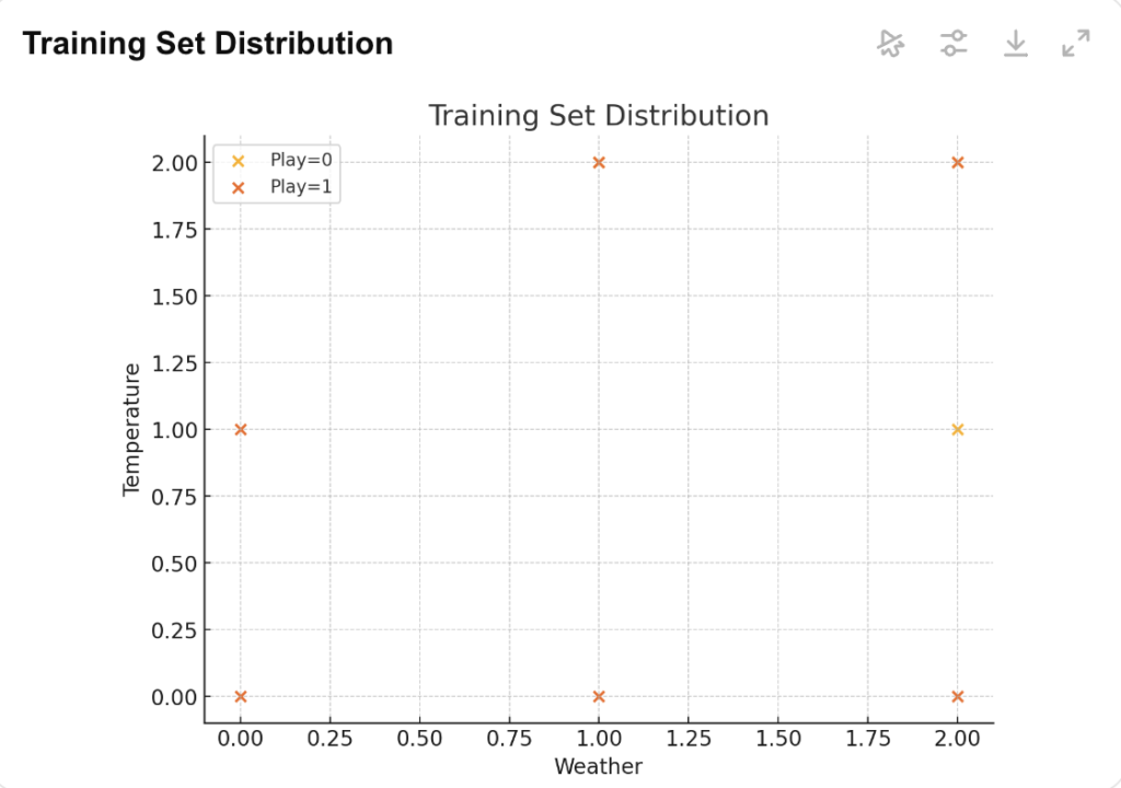
Visualization helps in understanding how the model performs on the training data. Since this is a simple example, we can plot the distribution of the data points.

Visualizing the Training Data Distribution

We’ll use matplotlib to create a scatter plot of the weather and temperature, with different colors representing whether playing is possible or not.

import matplotlib.pyplot as plt

# Plot the training set result
for label in [0, 1]:
    subset = X_train[y_train == label]
    plt.scatter(subset['Weather'], subset['Temperature'], label=f'Play={label}')

plt.xlabel('Weather')
plt.ylabel('Temperature')
plt.title('Training Set Distribution')
plt.legend()
plt.show()

This plot will give a visual representation of how the weather and temperature conditions affect the outcome of playing outside.

Visualizing the Test Set Result

Similarly, we can plot the test set predictions to see how well the model performed.

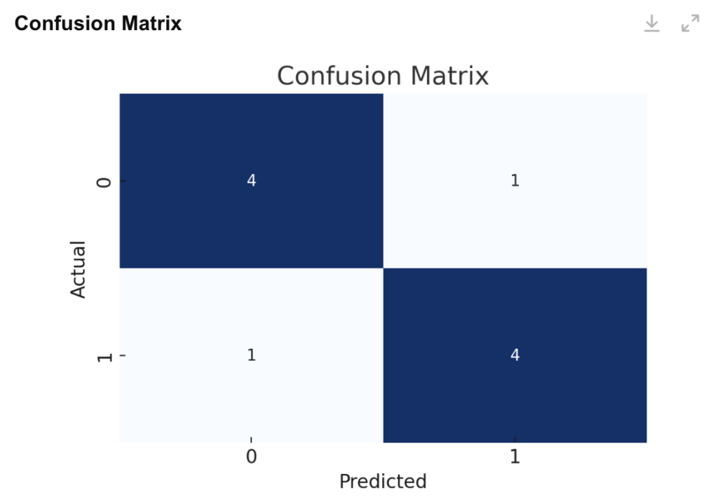
Plotting the Confusion Matrix for Test Data

A confusion matrix is a great way to visualize the performance of a classification model. Here, we’ll use seaborn for a cleaner visualization.

import seaborn as sns

# Plot confusion matrix
sns.heatmap(conf_matrix, annot=True, cmap='Blues', fmt='d', cbar=False)
plt.xlabel('Predicted')
plt.ylabel('Actual')
plt.title('Confusion Matrix')
plt.show()

This plot shows how many predictions were correct and how many were misclassified.

Conclusion

The Naive Bayes classifier is a simple yet powerful algorithm for solving classification problems. Despite its naive assumption of feature independence, it performs remarkably well for tasks like spam filtering, sentiment analysis, and document classification. The algorithm is particularly effective with high-dimensional data and works well even with small datasets.

However, it may struggle when the independence assumption is violated or when working with continuous features that don’t follow a normal distribution. Techniques like Laplace Smoothing help address the zero-probability issue, making it more robust.

In summary, Naive Bayes remains a fundamental algorithm in machine learning. Its simplicity, speed, and effectiveness make it a great choice for beginners, while its real-world applications highlight its practical value. Learning how to implement Naive Bayes is a solid step toward mastering classification algorithms.