The K-Nearest Neighbor (KNN) algorithm is one of the simplest yet powerful supervised learning techniques used for classification and regression tasks in machine learning. Understanding KNN is crucial for beginners as it provides insights into core concepts such as distance metrics and data point classification. This guide covers its mechanism, benefits, and real-world applications.
What is the K-Nearest Neighbor (KNN) Algorithm?
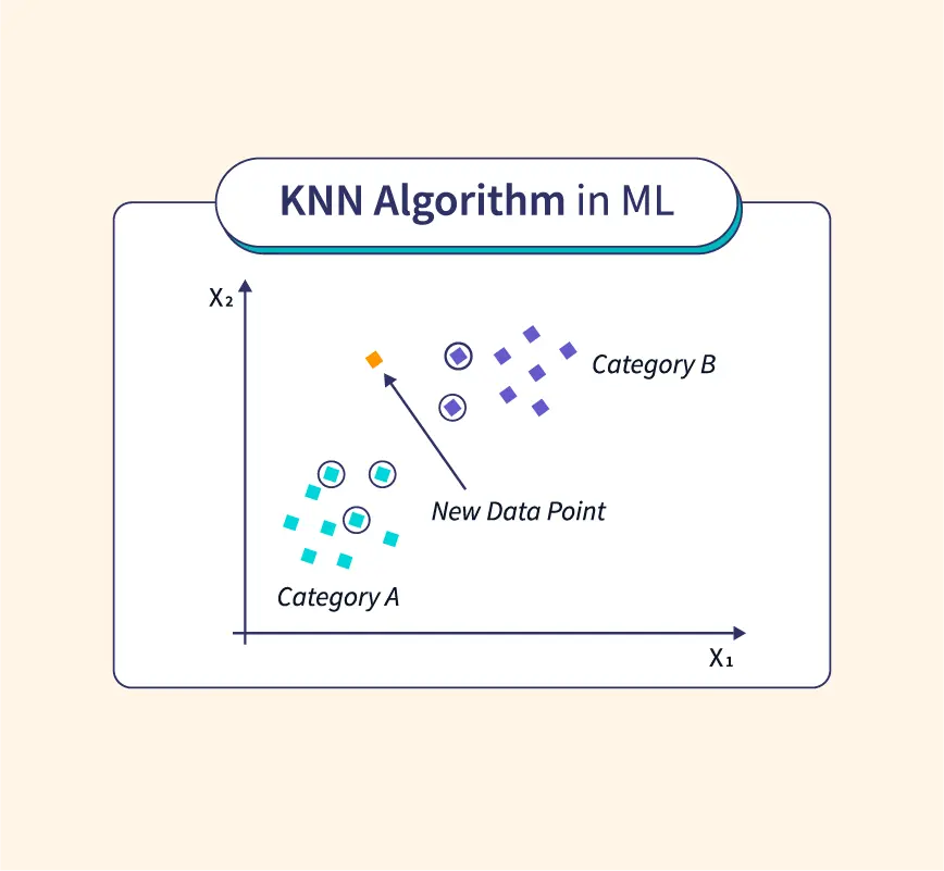
K-Nearest Neighbor (KNN) is a supervised learning algorithm used for both classification and regression. It is non-parametric, meaning it doesn’t make any assumptions about the underlying data distribution, which makes it versatile for various applications. KNN works by analyzing the proximity or “closeness” of data points based on specific distance metrics.
Source: SCALER
In classification, KNN assigns a class label to a new data point based on the majority class of its nearest neighbors. For instance, if a data point has five nearest neighbors, and three of them belong to class A while two belong to class B, the algorithm will classify the point as class A.
In regression, KNN predicts continuous values by averaging the values of the k-nearest neighbors. For example, if you’re predicting house prices, KNN will use the average prices of the k-nearest neighbors to estimate the price of a new house.
Types of Problems Solved by KNN
- Classification: Identifying which category a new observation belongs to.
- Regression: Predicting a continuous outcome based on similar observations.
KNN is widely used due to its simplicity and effectiveness in both small datasets and non-linear data distributions.
How Does KNN Work?
The KNN algorithm follows a straightforward, step-by-step approach:
Step 1: Determine the Number of Nearest Neighbors (k)
The first step is to select the number of neighbors (k) to consider. The value of k determines how many neighboring points will influence the classification or prediction of a new data point.
Step 2: Calculate the Distance Between the Query Point and Dataset Points
For each data point in the dataset, the algorithm calculates the distance between the query point (the new point to be classified or predicted) and every other point. Various distance metrics can be used, such as Euclidean distance, Manhattan distance, or Minkowski distance.
Step 3: Sort and Select the k-Nearest Neighbors
After calculating the distances, the algorithm sorts all data points in ascending order of distance. It then selects the k-nearest neighbors—the data points that are closest to the query point.
Step 4: Make a Prediction
- For classification: The algorithm assigns the query point to the class label that is most frequent among the k-nearest neighbors (majority voting).
- For regression: The algorithm predicts the value by averaging the values of the k-nearest neighbors.
Example:
Consider a dataset of three categories of fruits: apples, oranges, and bananas. When a new fruit data point is introduced, KNN will classify it by identifying the closest neighbors and determining the majority label among them.
KNN’s simplicity and intuitive working mechanism make it a popular choice for beginners to understand fundamental machine learning concepts.
How to Select the Value of K in the K-NN Algorithm?
Choosing the correct value of k is critical to the performance of the KNN algorithm. A small k value can make the model too sensitive to noise, resulting in overfitting, while a large k value can oversimplify the model, causing underfitting.
Methods to Select the Optimal k:
- Cross-Validation: A commonly used technique for choosing the value of k is cross-validation. By splitting the dataset into training and validation sets and evaluating model performance across different values of k, the optimal k value can be determined based on which k produces the lowest error rate.
- Common Values of k: In practice, values of k such as 3, 5, or 7 are typically chosen. Smaller values of k allow the model to capture local patterns, while larger k values generalize better across the dataset.
Impact on Model Performance:
- Too small k (e.g., k = 1): The model is highly sensitive to individual data points, leading to overfitting, as the prediction is based on just one point.
- Too large k: When k is too large, the model can become too smooth, losing important patterns in the data, leading to underfitting.
In summary, selecting an appropriate k value ensures the balance between model complexity and predictive accuracy.
Distance Metrics Used in KNN Algorithm
Distance metrics are crucial for calculating the similarity between data points in KNN. Here are the commonly used metrics:
1. Euclidean Distance
Euclidean distance is the most common distance metric, calculated as the straight-line distance between two points in Euclidean space. For two points $P(x_1, y_1)$ and $Q(x_2, y_2)$, the Euclidean distance is calculated as:
$$d(P,Q) = \sqrt{(x_2 – x_1)^2 + (y_2 – y_1)^2}$$
Euclidean distance is suitable for continuous variables and is easy to compute, making it a popular choice in KNN.
2. Manhattan Distance
Manhattan distance (or L1 distance) measures the distance between two points along the axes at right angles. For two points $P(x_1, y_1)$ and $Q(x_2, y_2)$, the Manhattan distance is calculated as:
$$d(P,Q) = |x_2 – x_1| + |y_2 – y_1|$$
It is useful for grid-like paths (e.g., city blocks) and is often employed when variables are more discrete.
3. Minkowski Distance
Minkowski distance is a generalization of both Euclidean and Manhattan distances. It is defined as:
$$d(P, Q) = \left( \sum_{i=1}^{n} |x_i – y_i|^p \right)^{1/p}$$
When $p = 2$, it becomes Euclidean distance, and when $p = 1$, it is equivalent to Manhattan distance. Minkowski distance provides flexibility by adjusting the value of $p$ for different scenarios.
Choosing the appropriate distance metric depends on the data type and the specific problem at hand.
Algorithm for K-Nearest Neighbor (KNN)
Here’s a simplified version of the KNN algorithm:
Algorithm Steps:
- Select the number of neighbors k.
- Calculate the distance between the query point and all other points in the dataset using a chosen distance metric.
- Sort the distances in ascending order and select the top k-nearest neighbors.
- For classification: Assign the query point the class of the majority of its neighbors.
- For regression: Predict the value of the query point as the average of the k-nearest neighbors.
Pseudo-code:
def knn(query_point, dataset, k):

    distances = []

    for point in dataset:

        distance = compute_distance(query_point, point)

        distances.append((point, distance))

    distances.sort(key=lambda x: x[1])  # Sort based on distance

    neighbors = distances[:k]

    prediction = majority_vote(neighbors)  # or average for regression

    return prediction
This simple algorithm shows the core logic of KNN, making it easy to implement and understand.
Advantages of KNN Algorithm
1. Simplicity and Ease of Implementation
KNN is easy to understand and implement. It doesn’t require complex parameter tuning or assumptions about data distribution.
2. Non-Parametric Nature
KNN is a non-parametric algorithm, meaning it does not assume any specific form for the underlying data. This makes it flexible and effective for a wide range of data types, including non-linear datasets.
3. Versatility
KNN can be used for both classification and regression, making it a versatile tool for machine learning applications.
4. Robustness to Noisy Data
KNN is relatively robust to noisy data, as the decision is based on multiple neighbors, not just a single data point. This reduces the effect of outliers on predictions.
Overall, KNN remains a valuable algorithm for many machine learning applications, particularly where simplicity and interpretability are important.
Disadvantages of KNN Algorithm
Despite its simplicity, KNN has several drawbacks:
1. Computational Inefficiency
KNN requires calculating the distance between the query point and every data point in the dataset. As the size of the dataset grows, this becomes computationally expensive and slow, particularly for large-scale applications.
2. Sensitivity to the Choice of k and Distance Metric
The performance of KNN depends heavily on the selection of k and the distance metric. Poor choices can lead to inaccurate predictions or overfitting/underfitting.
3. Storage-Intensive
KNN is a lazy learner, meaning it does not generalize from the training data before making predictions. It requires storing the entire dataset, which can lead to high memory usage, especially for large datasets.
4. Struggles with Imbalanced Data
In classification tasks, KNN struggles when there is an imbalance in the data classes. For example, if one class is overrepresented, it can dominate the voting process, leading to biased predictions.
Despite these limitations, KNN remains a useful algorithm for specific applications, especially when the dataset is small or moderately sized.
Applications of KNN Algorithm in Machine Learning
KNN is widely applied across various fields due to its simplicity and flexibility. Some of the key applications include:
1. Text Classification
KNN is often used for text classification tasks such as spam detection or document categorization. By analyzing the frequency of keywords and their similarity to previously labeled documents, KNN can classify new texts effectively.
2. Image Recognition
KNN is utilized in image recognition tasks where patterns within images can be identified based on pixel similarity. For instance, it can classify handwritten digits or recognize faces by comparing the pixel distributions.
3. Recommendation Systems
In recommendation engines, KNN is used to suggest products, movies, or content based on the preferences of similar users. By finding the nearest neighbors in user preferences, KNN can recommend items that are highly relevant to individual users.
4. Medical Diagnosis
KNN is applied in medical diagnosis to predict patient outcomes based on medical histories. By comparing a patient’s data with similar cases, the algorithm can provide recommendations for treatment or predict disease likelihood.
These applications showcase KNN’s versatility in handling diverse machine learning tasks.
Python Implementation of the KNN Algorithm
KNN Classification Example (Python using scikit-learn)
from sklearn.neighbors import KNeighborsClassifier

from sklearn.model_selection import train_test_split

from sklearn.datasets import load_iris

from sklearn.metrics import accuracy_score

# Load dataset

iris = load_iris()

X, y = iris.data, iris.target

# Split dataset into training and testing sets

X_train, X_test, y_train, y_test = train_test_split(X, y, test_size=0.3, random_state=42)

# Initialize the KNN classifier with k=3

knn = KNeighborsClassifier(n_neighbors=3)

# Train the model

knn.fit(X_train, y_train)

# Make predictions

y_pred = knn.predict(X_test)

# Evaluate the model

accuracy = accuracy_score(y_test, y_pred)

print(f"Accuracy: {accuracy * 100:.2f}%")
Explanation:
In this example, we use the Iris dataset, a common dataset in machine learning. The KNeighborsClassifier is initialized with k=3, and the model is trained on a split of the dataset. The accuracy score is then calculated to evaluate model performance.
Conclusion
The K-Nearest Neighbor (KNN) algorithm is a foundational machine learning technique that offers simplicity and versatility for both classification and regression tasks. Despite some limitations such as computational inefficiency in large datasets, KNN remains a powerful tool for various applications, from text classification to image recognition. Its intuitive nature makes it an excellent choice for beginner data scientists looking to understand basic machine learning concepts. By experimenting with KNN, beginners can gain valuable insights into distance metrics, classification techniques, and the importance of data preprocessing in machine learning workflows.
References: