Entropy in Machine Learning

In machine learning, models need to make informed decisions based on data. For this, they rely on methods to measure uncertainty and randomness within a dataset. One of the key concepts used to quantify this uncertainty is entropy. Derived from information theory, entropy helps machine learning algorithms determine how to split data most effectively, thereby improving prediction accuracy.

Entropy plays a critical role in various machine learning algorithms, particularly in decision trees, where it is used to calculate information gain, a metric that guides the model to the best decision-making path. Understanding entropy is essential for mastering machine learning, especially in the context of classification tasks where uncertainty needs to be minimized for more accurate predictions.

What is Entropy in Machine Learning?

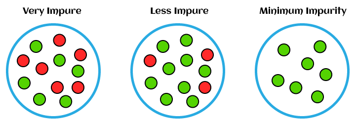
Entropy is a measure of uncertainty or randomness in a dataset. It originates from information theory, where it quantifies the amount of unpredictability or disorder within a set of data. In machine learning, entropy is used to calculate how mixed or impure a dataset is in terms of the target variable (such as class labels). The goal is to reduce entropy, thereby creating a model that makes more informed and accurate decisions.

In simpler terms, entropy helps us understand how uncertain we are about a particular event. A dataset with high entropy has a higher level of randomness and is more difficult to make predictions from, while a dataset with low entropy is more predictable and easier to classify.

For example, in a binary classification problem, if a dataset has an equal number of positive and negative examples, its entropy is high because it’s hard to predict the class of a randomly chosen instance. However, if the dataset contains mostly one class, the entropy is low since the outcome is more certain.

Entropy is foundational in decision tree algorithms, where it helps identify the feature that best splits the dataset by reducing uncertainty the most.

Mathematical Formula for Entropy

The mathematical formula for entropy, denoted by H, is derived from information theory and is given by:

Where:

• S is the set of data (or dataset),
• p(i) is the probability of class iii in the dataset S,
• n is the total number of classes (or unique labels),
• log₂​ is the logarithm base 2, used to measure information in bits.

Explanation of Variables:

• p(i): This represents the proportion of instances in the dataset that belong to class i. For example, in a binary classification problem, p(i) would represent the probability of an instance being classified as either class 1 or class 2.
• log_2 p(i): This is the information content or “surprise” factor of class i. The less probable an event is, the higher its information content.

The entropy formula essentially sums up the weighted information content of all classes in the dataset. When the dataset is pure (i.e., all instances belong to one class), entropy is zero. Conversely, when the classes are evenly distributed, the entropy is maximized.

Example:

Consider a dataset with two classes (binary classification), where:

• 60% of the examples belong to class 1 (p = 0.6),
• 40% belong to class 2 (p = 0.4).

The entropy of the dataset can be calculated as:

Calculating the values:

This entropy value of 0.971 indicates that the dataset has some level of uncertainty, though it’s not maximally uncertain.

What is a Decision Tree in Machine Learning?

A decision tree is a popular supervised learning algorithm used for both classification and regression tasks. It is a flowchart-like structure where each internal node represents a decision based on a feature, each branch represents an outcome of the decision, and each leaf node represents the final prediction or classification.

The key idea behind a decision tree is to split the data into subsets based on certain features. The splits are made in a way that reduces uncertainty (or entropy) in the dataset, making it easier to classify new data points accurately. Decision trees are non-parametric and handle both categorical and numerical data effectively.

Structure of a Decision Tree:

• Root Node: This is the top node of the tree, representing the entire dataset. The feature that provides the highest information gain (i.e., reduces entropy the most) is selected to split the data.
• Internal Nodes: These represent decision points where the dataset is split based on feature values. Each internal node tests a feature and splits the data into subsets based on the outcome.
• Leaf Nodes: These are the terminal nodes that represent the final prediction. Once the data reaches a leaf node, the model assigns a class label or regression value based on the data in that node.

Decision trees learn by recursively splitting the dataset based on features that maximize the reduction in entropy, ensuring that each split results in subsets that are as pure (homogeneous) as possible.

For example, in a decision tree for classifying whether an email is spam or not, the root node might test if the email contains certain keywords, and the branches would follow based on the presence or absence of these words, eventually leading to a classification.

Terminologies used in Decision Tree

Understanding the key terminologies associated with decision trees is essential for grasping how they work. Below are the most important terms:

• Root Node: The starting point of the decision tree, representing the entire dataset. At the root, the first split is made based on the feature that provides the highest information gain or best split criteria.
• Internal Node: A node where the dataset is split further based on a feature’s value. Each internal node represents a decision point where a question is asked, such as “Is the value of this feature greater than X?” The data is split based on the outcome of this decision.
• Leaf Node (Terminal Node): A leaf node is a terminal node that represents the final output or decision. Once the data reaches a leaf node, the model assigns a class label (in classification tasks) or a value (in regression tasks) based on the majority class or the mean value within that node.
• Branch (Edge): A path that connects a parent node to a child node. It represents the outcome of a decision made at an internal node. Each decision leads to a branch, directing the data to the next node.
• Splitting Criterion: The rule used to decide how to split the data at each internal node. Common splitting criteria include entropy, information gain, and Gini impurity. The goal is to split the data in such a way that the resulting subsets are more homogeneous, reducing uncertainty in the predictions.

Example:

In a decision tree for predicting whether a customer will purchase a product, the root node might ask, “Is the customer’s age greater than 30?” If the answer is yes, the data follows one branch; if no, it follows a different branch. The process continues through several internal nodes, making decisions based on features like income, previous purchase history, etc., until a leaf node is reached, where the model makes the final prediction.

Calculation of Entropy in Python

In this section, we’ll demonstrate how to calculate entropy in Python using a simple dataset. This can be particularly useful for those who want to understand how entropy works behind the scenes in machine learning algorithms like decision trees.

Below is a Python code snippet that calculates entropy for a binary classification problem:

import math

# Function to calculate the entropy of a dataset
def calculate_entropy(class_probabilities):
    """
    Calculate the entropy of a dataset given the probabilities of different classes.
    Args:
    class_probabilities: A list of probabilities for each class.
    
    Returns:
    Entropy value.
    """
    entropy = 0
    for prob in class_probabilities:
        if prob > 0:  # Only calculate for probabilities greater than 0
            entropy -= prob * math.log2(prob)
    return entropy

# Example: Class probabilities for a binary classification problem
# Let's assume we have two classes, with probabilities 0.6 and 0.4 respectively
class_probabilities = [0.6, 0.4]

# Calculate entropy
entropy_value = calculate_entropy(class_probabilities)
print(f"Entropy of the dataset: {entropy_value}")

Explanation of the Code:

1. Function Definition: The calculate_entropy function takes a list of class probabilities as input and returns the entropy value. It uses the entropy formula
   where p(i) is the probability of each class.

1. Class Probabilities: In the example, we have a binary classification dataset with two classes: one class has a probability of 0.6 and the other has a probability of 0.4.
2. Entropy Calculation: The function iterates over the class probabilities and applies the entropy formula to calculate the total entropy of the dataset.
3. Output: The entropy value of the dataset is printed, which, in this case, would be approximately 0.971, indicating some level of uncertainty in the dataset.

Use of Entropy in Decision Tree

Entropy plays a crucial role in decision trees by helping the algorithm determine how to split the dataset at each node to create the purest subsets of data. In decision trees, the goal is to reduce uncertainty as much as possible with each split, and this is where entropy comes into play.

Here’s how entropy is used in the decision tree building process:

Splitting the Data

• At each internal node, the decision tree evaluates the potential features that could be used to split the data. For each feature, the algorithm calculates the entropy of the target variable (e.g., class labels) before and after the split.
• The information gain (which we will cover in the next section) is computed by subtracting the entropy of the resulting child nodes from the entropy of the parent node. The feature that provides the greatest reduction in entropy (i.e., the largest information gain) is chosen to split the data at that node.

Example:

Suppose you are building a decision tree to classify whether customers will buy a product based on features like income and age. At the root node, the decision tree calculates the entropy for the target variable (buy/no-buy) based on the entire dataset. It then evaluates potential splits on features like income or age, calculating how much the entropy decreases after each split. The feature that reduces entropy the most is chosen to split the data at the root node.

Reducing Entropy for Purity

• The objective of each split in a decision tree is to create subsets of data that are more homogeneous in terms of the target variable (i.e., to have leaf nodes that contain data points mostly from a single class). When a node has zero entropy (i.e., all data points in that node belong to the same class), the node is “pure,” and no further splits are needed.

Summary:

• Entropy is used as a criterion for selecting features to split the data at each node in a decision tree.
• The algorithm aims to reduce entropy and create the purest possible subsets with each split.
• Lower entropy means more certainty in the prediction, which leads to more accurate decision-making in the tree.

What is the Information Gain in Entropy?

Information gain is a metric used in decision trees to measure how much entropy is reduced after splitting the dataset based on a particular feature. It helps determine the feature that provides the most valuable split at each step of building the tree.

Definition:

Information gain is the difference between the entropy of the parent node (before the split) and the weighted average entropy of the child nodes (after the split). The feature that results in the highest information gain is chosen for splitting the data.

Mathematical Formula:

The information gain IGIGIG is calculated as:

Where:

• IG(S,A) is the information gain for feature A,
• H(S) is the entropy of the dataset before the split,
• Sv​ is the subset of data where the feature A takes the value v,
• ∣Sv∣/∣S∣ is the weighted proportion of instances in Sv​ relative to the whole dataset,
• H(Sv​) is the entropy of the subset after the split.

Example:

Suppose we are building a decision tree to classify whether students pass or fail based on study hours. The entropy of the dataset (before the split) is calculated as H(S)=0.971

After splitting the data on the feature “study hours,” the algorithm calculates the entropy of the child nodes (let’s say, one child node has entropy H(S1)=0.5 and the other has entropy H(S2)=0.2

The information gain for this split can be calculated by subtracting the weighted average entropy of the child nodes from the parent node entropy:

The feature with the highest information gain will be selected for splitting the data.

Importance:

• Information gain helps the decision tree algorithm identify the most informative feature for splitting the dataset at each node.
• It ensures that each split contributes to reducing uncertainty (entropy) and increasing the model’s accuracy.

How to Build Decision Trees Using Information Gain

Building a decision tree using information gain involves a step-by-step process where the dataset is recursively split based on the feature that provides the highest information gain at each node. Here’s how you can build a decision tree:

Step-by-Step Process:

1. Start with the Entire Dataset (Root Node):

• Begin with the entire dataset at the root node. All data points are present at this level, and the initial entropy of the dataset is calculated.

2. Calculate Entropy for the Dataset:

• Compute the entropy of the target variable (e.g., class labels) for the entire dataset. This gives an idea of how uncertain the target classification is.

3. Calculate Information Gain for All Features:

• For each feature in the dataset, calculate the entropy for the child nodes that would result from splitting the dataset based on that feature.
• For each possible split, compute the weighted average entropy of the child nodes and subtract it from the entropy of the parent node to determine the information gain for that feature.

4. Choose the Feature with the Highest Information Gain:

• Select the feature that provides the highest information gain as the splitting criterion for the root node. This feature will reduce the uncertainty in the dataset the most.

5. Split the Data and Create Child Nodes:

• Split the dataset into subsets based on the values of the selected feature. Each subset corresponds to a child node in the decision tree. The goal is to make these child nodes as pure as possible (i.e., have low entropy).

6. Recursively Repeat the Process:

• For each child node, repeat the process: calculate the information gain for all features in that subset, select the feature with the highest information gain, and split the data again. This process continues until one of the stopping criteria is met.

7. Stopping Criteria:

• The recursion stops when:
  • The node becomes pure (entropy is zero, meaning all data points in the node belong to the same class).
  • There are no remaining features to split.
  • A predefined maximum tree depth is reached.

8. Assign Labels to Leaf Nodes:

• Once a node can no longer be split, it becomes a leaf node. Each leaf node represents a final classification. The class label is assigned based on the majority class in that node.

Example:

Consider building a decision tree to predict whether a customer will buy a product based on features like age and income. The algorithm starts by calculating the entropy of the target variable (buy/not buy). It then calculates the information gain for each feature, choosing the one that reduces entropy the most (e.g., “age”). The data is split based on “age,” and the process is repeated for the remaining features until the tree is built.

Advantages of Decision Trees

Decision trees are a popular machine learning algorithm due to their versatility and simplicity. Below are some of the key advantages of using decision trees:

1. Easy to Interpret and Visualize:

• Decision trees are highly intuitive, as the decision-making process can be easily understood by following the tree from the root to the leaves. The model’s logic is straightforward, making it easier for non-technical stakeholders to grasp how predictions are made.
• The tree structure is also simple to visualize, which helps in identifying the decision paths and understanding the impact of each feature.

2. Handles Both Numerical and Categorical Data:

• Decision trees are flexible enough to handle both continuous (numerical) and categorical features. This makes them suitable for a wide range of tasks without requiring complex pre-processing steps, like converting categorical variables into numerical formats.

3. No Need for Feature Scaling:

• Unlike algorithms like SVM or logistic regression, decision trees do not require feature scaling (e.g., normalization or standardization). This is because the model uses feature values to create splits rather than relying on distances, so the magnitude of the features doesn’t impact the splits.

4. Robust to Outliers:

• Decision trees are less sensitive to outliers compared to other machine learning algorithms. Since the splits are based on feature values that lead to the highest information gain, extreme values in the dataset tend not to significantly affect the structure of the tree.

5. Handles Missing Values:

• Decision trees can handle missing values in the data by assigning the missing values to the most likely class or by splitting the dataset based on available features. Some implementations of decision trees have built-in methods to deal with missing data.

6. Captures Non-linear Relationships:

• Decision trees can capture non-linear relationships between features and the target variable. They do not assume any predefined relationship between input variables and output, making them highly flexible for tasks where non-linear patterns exist.

7. Reduced Computational Complexity for Small to Medium-sized Data:

• For small to medium-sized datasets, decision trees are computationally efficient and can be trained relatively quickly. Their recursive splitting mechanism works well for such datasets.