Bootstrapping in Machine Learning

In machine learning, understanding and managing uncertainty is essential. When building models, we often face questions about how well a model will perform on new data or how accurate the estimates are. Bootstrapping in machine learning is a statistical resampling technique that helps address these uncertainties by generating multiple samples from the original dataset and analyzing the variability of outcomes.

Bootstrapping allows us to assess model performance, estimate variability, and gain insights into the stability of predictions. By repeatedly sampling data and evaluating results, we can build more robust and reliable models in machine learning

What is Bootstrapping?

Bootstrapping is a statistical method that involves creating multiple samples from a single dataset to estimate a model’s accuracy and stability. The key concept behind bootstrapping is sampling with replacement, which means that each sample drawn from the dataset can include duplicate entries. This allows us to create several “bootstrapped” datasets, each of which is slightly different from the original.

An easy way to think of bootstrapping is to imagine “pulling oneself up by one’s bootstraps”—in this case, we’re using the dataset itself to generate multiple samples without needing new data. Bootstrapping differs from other resampling methods, like cross-validation, as it focuses more on understanding model uncertainty rather than solely on model validation​

How to Use Bootstrapping in Machine Learning?

Bootstrapping has multiple applications in machine learning, helping practitioners better understand and improve their models. Here are some common uses:

• Estimating Model Performance: Bootstrapping allows us to estimate metrics like accuracy, precision, and recall by creating multiple samples and testing the model on each. This helps assess how well a model might perform on unseen data.
• Model Selection: Bootstrapping can assist in choosing the best model among several options by evaluating each model’s performance variability across bootstrapped datasets. It provides insight into which model is more stable and reliable.
• Feature Importance: Bootstrapping helps identify the most influential features in a dataset. By analyzing feature importance across multiple bootstrapped samples, we can see which features consistently impact the model’s predictions.

Bootstrapping in Calculating Mean

One simple way to understand bootstrapping is by using it to calculate the mean (average) of a dataset. Let’s say we want to estimate the average height of students in a school. Instead of collecting more data, we can create multiple bootstrapped samples from our original dataset of heights. Each sample is generated by randomly selecting values with replacement, meaning some heights may appear more than once in a sample.

For each bootstrapped sample, we calculate the mean height. By repeating this process, we get a range of mean values, allowing us to estimate the distribution of the mean and understand its variability. This approach helps in making more confident estimates of the true mean, especially with small datasets where direct calculation might not capture variability​.

Bootstrapping in Classification Task With a Decision Tree

What Is a Decision Tree?

A Decision Tree is a machine learning model that classifies data by splitting it into branches based on feature values. Here’s how it works:

• The tree starts with a root node that represents the entire dataset.
• At each node, the data is split based on specific features, creating branches that represent decisions.
• This process continues until the tree reaches a final decision or “leaf,” classifying the data point into a particular category.

Decision trees are popular for classification tasks because they’re intuitive, easy to interpret, and work well with both numerical and categorical data.

What Is the Iris Dataset?

The Iris dataset is a classic dataset used frequently in machine learning for demonstrating classification models. It contains 150 samples of iris flowers, each with the following features:

• Petal Length and Petal Width
• Sepal Length and Sepal Width
• Species: The target label, with three possible classes (Iris Setosa, Iris Versicolour, and Iris Virginica).

The goal is to classify each flower species based on its features. Because of its simplicity, the Iris dataset is ideal for testing and visualizing models like decision trees.

Code Example

import pandas as pd
import seaborn as sns
from sklearn.datasets import load_iris
import matplotlib.pyplot as plt

# Load the Iris dataset
iris = load_iris()
# Create a DataFrame with feature names
iris_df = pd.DataFrame(data=iris.data, columns=iris.feature_names)
# Add the target label
iris_df['species'] = iris.target

# Map the target labels to species names
species_map = {0: 'Iris Setosa', 1: 'Iris Versicolour', 2: 'Iris Virginica'}
iris_df['species'] = iris_df['species'].map(species_map)

# Display the first few rows of the dataset
print("First five rows of the Iris dataset:")
print(iris_df.head())

# Basic visualization - Pairplot of features by species
sns.pairplot(iris_df, hue="species", markers=["o", "s", "D"])
plt.suptitle("Iris Dataset Feature Distributions by Species", y=1.02)
plt.show()

Explanation

1. Load and Prepare the Data: We load the Iris dataset and convert it into a pandas DataFrame. We also map the target labels (0, 1, and 2) to the species names for better readability.
2. Display Sample Data: We print the first five rows to get an overview of the dataset’s structure, showing features like petal and sepal dimensions, along with the species label.
3. Visualize the Features: We use Seaborn’s pairplot to visualize the relationships between features (e.g., petal length and width) by species. This plot helps illustrate how the features vary across the different species.

Example Output

sepal length (cm)	sepal width (cm)	petal length (cm)	petal width (cm)	species
5.1	3.5	1.4	0.2	Iris Setosa
4.9	3	1.4	0.2	Iris Setosa
4.7	3.2	1.3	0.2	Iris Setosa
4.6	3.1	1.5	0.2	Iris Setosa
5	3.6	1.4	0.2	Iris Setosa

Bootstrapping Visualization

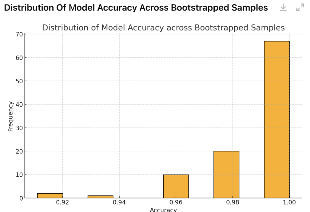
Bootstrapping can help visualize the distribution of model performance by repeatedly training a decision tree on different bootstrapped samples of the dataset. Here’s how we can approach it:

• Train on Multiple Samples: By applying bootstrapping, we create multiple bootstrapped datasets from the original data and train a decision tree on each sample.
• Record Performance: For each bootstrapped model, we calculate a performance metric, such as accuracy.
• Plot the Results: Plotting these accuracy scores on a histogram shows the range and variability in model performance across samples.

This visualization helps us understand how consistently the model performs and if its accuracy varies significantly depending on the sample.

Code Example

import numpy as np
from sklearn.tree import DecisionTreeClassifier
from sklearn.datasets import load_iris
from sklearn.utils import resample
from sklearn.model_selection import train_test_split
from sklearn.metrics import accuracy_score
import matplotlib.pyplot as plt

# Load the Iris dataset
data = load_iris()
X, y = data.data, data.target

# Split the data into training and testing sets
X_train, X_test, y_train, y_test = train_test_split(X, y, test_size=0.3, random_state=42)

# Set up bootstrapping parameters
n_iterations = 100  # Number of bootstrapped samples
accuracies = []

# Bootstrapping loop: train and record accuracy on each sample
for i in range(n_iterations):
    # Create a bootstrapped sample of the training data
    X_resampled, y_resampled = resample(X_train, y_train, replace=True)
    
    # Initialize and train the Decision Tree Classifier
    model = DecisionTreeClassifier()
    model.fit(X_resampled, y_resampled)
    
    # Predict on the test set
    y_pred = model.predict(X_test)
    
    # Calculate accuracy and store it
    accuracy = accuracy_score(y_test, y_pred)
    accuracies.append(accuracy)

# Plotting the distribution of accuracies from bootstrapped samples
plt.hist(accuracies, bins=10, edgecolor='black')
plt.title("Distribution of Model Accuracy across Bootstrapped Samples")
plt.xlabel("Accuracy")
plt.ylabel("Frequency")
plt.show()

Explanation

1. Bootstrapping Process: We loop through a specified number of iterations, creating a new bootstrapped sample of the training data each time and training a decision tree on that sample.
2. Record Performance: For each trained model, we evaluate its accuracy on a fixed test set and store the accuracy score.
3. Plot Results: Using matplotlib, we plot the distribution of accuracy scores on a histogram. This visualization reveals the range of model performance across bootstrapped samples, helping us understand the variability in accuracy.

Example Output

Reproducing Best Results

Bootstrapping also plays a critical role in assessing the stability and reliability of a model:

• Identify Stability Issues: Training a model on different bootstrapped datasets can reveal if it performs inconsistently, indicating instability.
• Combine Models: To improve stability, techniques like ensemble methods (such as bagging) combine multiple bootstrapped models, helping to smooth out variability.
• Adjust Model Settings: By analyzing performance across samples, we can refine model parameters or adjust features to improve robustness.

Implementing Bootstrapping in Python

Let’s walk through a simple example to see how bootstrapping can be applied in Python using scikit-learn and NumPy. In this example, we’ll use bootstrapping to create multiple samples from a dataset and estimate the accuracy of a model.

import numpy as np
from sklearn.tree import DecisionTreeClassifier
from sklearn.datasets import load_iris
from sklearn.utils import resample
from sklearn.model_selection import train_test_split
from sklearn.metrics import accuracy_score

# Load the Iris dataset
data = load_iris()
X, y = data.data, data.target

# Splitting the data into training and testing sets
X_train, X_test, y_train, y_test = train_test_split(X, y, test_size=0.3, random_state=42)

# Bootstrapping parameters
n_iterations = 100  # Number of bootstrapped samples
bootstrapped_accuracies = []

# Bootstrapping loop
for i in range(n_iterations):
    # Resample the training data with replacement
    X_resampled, y_resampled = resample(X_train, y_train, replace=True)
    
    # Initialize and train the Decision Tree Classifier
    model = DecisionTreeClassifier()
    model.fit(X_resampled, y_resampled)
    
    # Predict on the test set
    y_pred = model.predict(X_test)
    
    # Calculate accuracy and store it
    accuracy = accuracy_score(y_test, y_pred)
    bootstrapped_accuracies.append(accuracy)

# Calculate the mean and standard deviation of the bootstrapped accuracies
mean_accuracy = np.mean(bootstrapped_accuracies)
std_dev_accuracy = np.std(bootstrapped_accuracies)

print("Bootstrapped Mean Accuracy:", mean_accuracy)
print("Accuracy Standard Deviation:", std_dev_accuracy)

Explanation

• Data Preparation: We load the Iris dataset and split it into training and testing sets.
• Bootstrapping Loop: For each iteration, we create a new bootstrapped sample of the training data and train a Decision Tree classifier on it.
• Performance Calculation: We test the model on the fixed test set and calculate its accuracy, recording the accuracy score in each iteration.
• Results Summary: Finally, we calculate the mean and standard deviation of the accuracy scores across all bootstrapped samples, giving us an estimate of the model’s performance and its variability.

Output (Example)

Bootstrapped Mean Accuracy: 0.94
Accuracy Standard Deviation: 0.02

This output shows the average accuracy and the standard deviation, indicating how stable the model’s performance is across bootstrapped samples.

Advantages and Disadvantages of Bootstrapping

Bootstrapping is a powerful and versatile tool in machine learning, but it has both strengths and limitations. Here’s a quick look at its pros and cons:

Advantages

• Simple to Implement: Bootstrapping is relatively easy to understand and apply. It requires no complex setup, making it accessible for beginners and advanced users alike.
• No Assumptions About Data Distribution: Unlike some statistical methods, bootstrapping doesn’t assume a specific distribution for the data, allowing it to be used in a wide range of scenarios.
• Estimates Model Uncertainty: By generating multiple samples, bootstrapping helps assess the variability and stability of model performance, giving valuable insights into model reliability.

Disadvantages

• Computationally Intensive: Bootstrapping can be resource-intensive, especially with large datasets or many iterations, as it requires training multiple models on different samples.
• Not Suitable for All Data Types: Bootstrapping may not work well for data with strong temporal or spatial dependencies (e.g., time series data), where the order or location of data points matters.
• Limited for Small Datasets: With very small datasets, bootstrapping may lead to biased results since repeated sampling from limited data might not capture the full variability.

Conclusion

Bootstrapping is an invaluable technique in machine learning for understanding model performance and addressing uncertainty. By generating multiple samples from the same dataset, bootstrapping helps estimate metrics like accuracy and feature importance, providing insights into model reliability and stability. It’s straightforward to implement and doesn’t rely on strict data distribution assumptions, making it a versatile tool.

However, bootstrapping isn’t suitable for all situations. It can be computationally demanding and may not work well with small datasets or data with dependencies like time series. Despite these limitations, bootstrapping remains a key method for building robust and trustworthy models, supporting decisions across a wide range of machine learning applications.